Capturing spontaneous partitioning of peripheral proteins using a biphasic membrane-mimetic model
By Mark J Arcario, Y Zenmei Ohkubo, Emad Tajkhorshid, and Ingo H Greger
Published in The journal of physical chemistry B 115(21): 7029-37 on June 2, 2011.
PMID: 21561114. PMCID: PMC3102442. Link to Pubmed page.
Core Facility: Computational Modeling
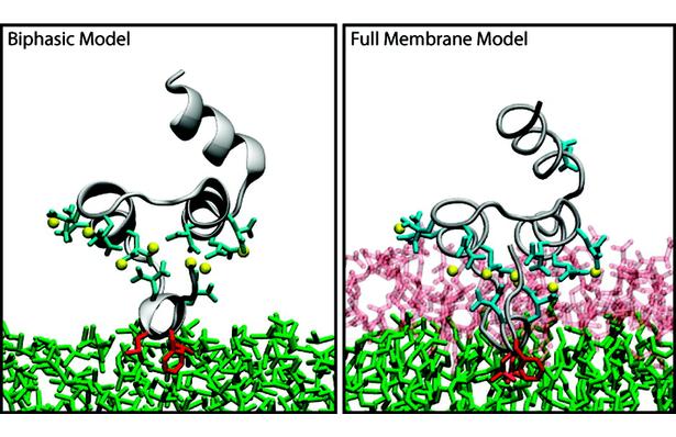
The biphasic system can be used to efficiently identify how deep the protein penetrates into the membrane’s hydrophobic core, thereby providing a guide for placement and modeling of the protein in a full membrane system. By aligning the interfacial region of the full lipid bilayer to the aqueous–organic interface in the biphasic model, one can maximize the overlap between the hydrophobic regions of the two representations, thus ensuring an optimal initial insertion of the protein into the hydrophobic core of the full membrane.
Abstract
Membrane binding of peripheral proteins, mediated by specialized anchoring domains, is a crucial step for their biological function. Computational studies of membrane insertion, however, have proven challenging and largely inaccessible, due to the time scales required for the complete description of the process, mainly caused by the slow diffusion of the lipid molecules composing the membrane. Furthermore, in many cases, the nature of the membrane “anchor”, i.e., the part of the protein that inserts into the membrane, is also unknown. Here, we address some of these issues by developing and employing a simplified representation of the membrane by a biphasic solvent model which we demonstrate can be used efficiently to capture and describe the process of hydrophobic insertion of membrane anchoring domains in all-atom molecular dynamics simulations. Applying the model, we have studied the insertion of the anchoring domain of a coagulation protein (the GLA domain of human protein C), starting from multiple initial configurations varying with regard to the initial orientation and height of the protein with respect to the membrane. In addition to efficiently and consistently identifying the “keel” region as the hydrophobic membrane anchor, within a few nanoseconds each configuration simulated showed a convergent height (2.20 ± 1.04 Å) and angle with respect to the interface normal (23.37 ± 12.48°). We demonstrate that the model can produce the same results as those obtained from a full representation of a membrane, in terms of both the depth of penetration and the orientation of the protein in the final membrane-bound form with an order of magnitude decrease in the required computational time compared to previous models, allowing for a more exhaustive search for the correct membrane-bound configuration.

 Plot of the self-diffusion coefficients D calculated for each species as a function of the time interval Δt; (Right) Molecular images of the organic species tested.")

 and water (dashed curve) phases averaged over the simulation period of 2 ns. The dotted line at x = 0 represents the approximate location of the DCLE/water interface.")

 The height of the keel Cα atoms above the DCLE/water interface, which was assumed to be the average position of the first layer of DCLE molecules in contact with water. (Bottom) The angle between the GLA domain’s axis, determined by the vector traced from the Ca2+-4 and the Cα of Phe40 (see Figure 1), and the interface normal (z-axis).")

